Discretization Animation

In this example, we create an animation of the right-most part of the spectrum obtained via method proposed in [Jarlebring et al., 2010]. The considered system is the following retarded delay differential equation (RDDE) from [Verheyden et al., 2008] Section 6.1:

\[\begin{split}\dot{x}(t) = \begin{bmatrix} -1 & 0 & 0 & 0 \\ 0 & 1 & 0 & 0 \\ 0 & 0 & -10 & -4 \\ 0 & 0 & 4 & -10 \end{bmatrix} x(t) + \begin{bmatrix} 3 & 3 & 3 & 3\\ 0 & -1.5 & 0 & 0 \\ 0 & 0 & 3 & -5 \\ 0 & 5 & 5 & 5 \end{bmatrix} x(t-1).\end{split}\]

import numpy as np
import matplotlib.pyplot as plt
import matplotlib.animation as animation

import tdcpy
import tdcpy.plot

# Create RDDE matrix representation
A0 = np.array([[-1, 0, 0, 0],
               [0, 1, 0, 0],
               [0, 0, -10, -4],
               [0, 0, 4, -10]])
A1 = np.array([[3, 3, 3, 3],
               [0, -1.5, 0, 0],
               [0, 0, 3, -5],
               [0, 5, 5, 5]])
rdde = tdcpy.RDDE(A=[A0, A1], hA=[0, 1])

/home/runner/work/tdcpy/tdcpy/src/tdcpy/ddae.py:32: SyntaxWarning: invalid escape sequence '\d'
  E \dot{x}(t) = \sum_{k=1}^{m_A} A_k x(t - h_{A,k})
/home/runner/work/tdcpy/tdcpy/src/tdcpy/common/delay_difference_equation.py:47: SyntaxWarning: invalid escape sequence '\d'
  E \dot{x}(t) = A_0 x(t - h_{A,0}) + ... + A_{m_A} x(t - h_{A,m_A})
/home/runner/work/tdcpy/tdcpy/src/tdcpy/rdde.py:24: SyntaxWarning: invalid escape sequence '\d'
  \dot{x}(t) = \sum_{k=1}^{m_A} A_k x(t - h_{A,k})
/home/runner/work/tdcpy/tdcpy/src/tdcpy/common/composition.py:72: SyntaxWarning: invalid escape sequence '\d'
  E \dot{x}(t) &= A_0 x(t - h_{A,0}) + ... + A_{n} x(t - h_{A,n}) +
/home/runner/work/tdcpy/tdcpy/src/tdcpy/stability/characteristic_roots.py:53: SyntaxWarning: invalid escape sequence '\d'
  E \dot{x}(t) = \sum\limits_{k=1}^N x(t-h_{A,k})  \ldots \qquad (1)
/home/runner/work/tdcpy/tdcpy/src/tdcpy/stability/characteristic_roots.py:406: SyntaxWarning: invalid escape sequence '\d'
  E \dot{x}(t) = \sum\limits_{k=1}^N A_k x(t-h_{A,k})
/home/runner/work/tdcpy/tdcpy/src/tdcpy/common/discretization.py:35: SyntaxWarning: invalid escape sequence '\d'
  E \dot{x}(t) = A_0 x(t) + A_1 x(t - h_{A,1}) + ... + A_{m} x(t - h_{A,m}),
/home/runner/work/tdcpy/tdcpy/src/tdcpy/stability/discretization_heuristic.py:158: SyntaxWarning: invalid escape sequence '\P'
  \Psi, default 20
/home/runner/work/tdcpy/tdcpy/src/tdcpy/stability/newton.py:37: SyntaxWarning: invalid escape sequence '\e'
  v0.H &0      \end{bmatrix}

to be determined by the heuristic. It is possible to access the discretization and also raw eigenvalues of constructed eigenvalue problem from info.

roots, info = tdcpy.roots(rdde, r=-2)
print(f"N = {info.discretization}")
print(f"First 5 raw eigenvalues: {info.discretization_eigenvalues[:5]}")

N = 30
First 5 raw eigenvalues: [-256.68292389-236.9936388j  -256.68292389+236.9936388j
  -31.95257255-186.96261937j  -31.95257255+186.96261937j
  -17.63828644-124.58864958j]

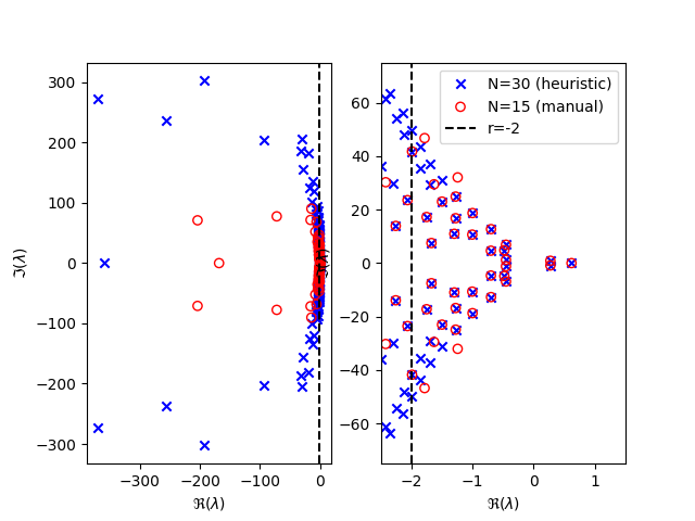
discretization eigenvalues for both cases.

roots2, info2 = tdcpy.roots(rdde, r=-2, discretization=15)

fix, (ax1, ax2) = plt.subplots(1, 2)

tdcpy.plot.complex_scatter_axplot(info.discretization_eigenvalues, ax=ax1,
                                  marker="x", color="b")
tdcpy.plot.complex_scatter_axplot(info2.discretization_eigenvalues, ax=ax1,
                                  marker="o", edgecolors="r", facecolors='none')
ax1.axvline(x=-2, color="k", linestyle="--", label="r=-2")
ax1.set_xlabel(r"$\Re (\lambda)$")
ax1.set_ylabel(r"$\Im (\lambda)$")

tdcpy.plot.complex_scatter_axplot(info.discretization_eigenvalues, ax=ax2,
                                  marker="x", color="b",
                                  label=f"N={info.discretization} (heuristic)")
tdcpy.plot.complex_scatter_axplot(info2.discretization_eigenvalues, ax=ax2,
                                  marker="o", edgecolors="r", facecolors='none',
                                  label=f"N={info2.discretization} (manual)")
ax2.axvline(x=-2, color="k", linestyle="--", label="r=-2")
ax2.set_xlim(-2.5, 1.5)
ax2.set_ylim(-75, 75)
ax2.set_xlabel(r"$\Re (\lambda)$")
ax2.set_ylabel(r"$\Im (\lambda)$")
ax2.legend()

plt.show()

We use the build-in function for creating the discretization animation. If further customization would be needed, we encourage to read the source code of tdcpy.plot.discretization_animation(.) and adapt it.

ani = tdcpy.plot.discretization_animation(
    rdde,
    s0=0,
    discretization=range(10, 100, 5),
    discretization_ideal=120,
    xlim=(-5.25, 1.5),
    ylim=(-200, 200),
    interval=200,
)
ani.save("discretization.gif", writer="pillow")

Once Loop Reflect