Prelude to strong stability - gradient of \(c_D\)

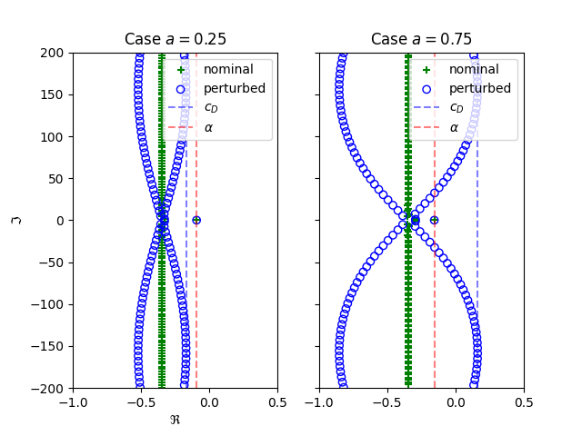
First, we consider Example 13 from [Michiels, 2011]

\[\begin{split}\begin{bmatrix} 1 & 0\\ 0 & 0 \end{bmatrix} \dot{x}(t) = \begin{bmatrix} 0 & -\frac{1}{8}\\ -1 & 1 \end{bmatrix} x(t) + \begin{bmatrix} 0 & 0\\ 0 & -a \end{bmatrix} x(t-\tau_1) + \begin{bmatrix} 0 & 0\\ 0 & \frac{1}{2} \end{bmatrix} x(t-\tau_2)\end{split}\]

and show that for certain values of \(a\) the system is not strongly stable. Next, we show how dradient of spectral abscissa of associated delay-difference equation can be computed and used to obtain strong stability.

import numpy as np
import matplotlib.pyplot as plt
from scipy import linalg

import tdcpy
import tdcpy.plot

# Define system descriptor matrices
E = np.array([
    [1, 0.],
    [0, 0],
])
A0 = np.array([
    [0, -1./8],
    [-1, 1],
])
A1 = np.array([
    [0, 0],
    [0, -0.25],
])
A2 = np.array([
    [0, 0],
    [0, 0.5],
])

# Create DDAE systems with a=0.25 with tau1=1 and tau1=0.99
ddae1 = tdcpy.DDAE(A=[A0, A1, A2], hA=np.array([0, 1, 2]), E=E)
ddae1_perturbed = tdcpy.DDAE(A=[A0, A1, A2], hA=np.array([0, 0.99, 2]), E=E)

# Create DDAE systems with a=0.75 with tau1=1 and tau1=0.99
A1[1,1] = -0.75
ddae2 = tdcpy.DDAE(A=[A0, A1, A2], hA=np.array([0, 1, 2]), E=E)
ddae2_perturbed = tdcpy.DDAE(A=[A0, A1, A2], hA=np.array([0, 0.99, 2]), E=E)

region = [-1, 0.5, -200, 200]

# Solve a=0.25
cr1, _ = tdcpy.roots(ddae1, r=region)
cr1_perturbed, _ = tdcpy.roots(ddae1_perturbed, r=region)
sa1 = tdcpy.sa(ddae1)
cd1, _ = tdcpy.cd(ddae1)

# solve a=0.75
cr2, _ = tdcpy.roots(ddae2, r=region)
cr2_perturbed, _ = tdcpy.roots(ddae2_perturbed, r=region)
sa2 = tdcpy.sa(ddae2)
cd2, _ = tdcpy.cd(ddae2)

fig, (ax1, ax2) = plt.subplots(1,2, sharex=True, sharey=True)

ax1.set_title("Case $a=0.25$")
tdcpy.plot.complex_scatter_axplot(cr1, ax=ax1, marker="+", color="green", label="nominal")
tdcpy.plot.complex_scatter_axplot(cr1_perturbed, ax=ax1, marker="o", edgecolor="blue", facecolor="none", label="perturbed")
ax1.axvline(x=cd1, color='b', linestyle='--', alpha=0.5, label=r"$c_D$")
ax1.axvline(x=sa1, color='r', linestyle='--', alpha=0.5, label=r"$\alpha$")
ax1.set_xlabel(r"$\Re$")
ax1.set_ylabel(r"$\Im$")
ax1.set_xlim(region[0], region[1])
ax1.set_ylim(region[2], region[3])
ax1.legend()

ax2.set_title("Case $a=0.75$")
tdcpy.plot.complex_scatter_axplot(cr2, ax=ax2, marker="+", color="green", label="nominal")
tdcpy.plot.complex_scatter_axplot(cr2_perturbed, ax=ax2, marker="o", edgecolor="blue", facecolor="none", label="perturbed")
ax2.axvline(x=cd2, color='b', linestyle='--', alpha=0.5, label=r"$c_D$")
ax2.axvline(x=sa2, color='r', linestyle='--', alpha=0.5, label=r"$\alpha$")
ax1.set_xlabel(r"$\Re$")
ax1.set_ylabel(r"$\Im$")
ax2.set_xlim(region[0], region[1])
ax2.set_ylim(region[2], region[3])
ax2.legend()

plt.show()

Next, let us show how gradient of \(c_D\) can be computed and used to

minimize \(c_D\) and obtain strong stability (assuming right most root is stable).

We are going to proceed manually, i.e. follow preciselly the equations in TODO

%%

# step one, obtain U and V
uE = linalg.null_space(E.T)
vE = linalg.null_space(E)

# step two, obtain D0, D1, D2, observe that D1 can be written by - a B C
B = np.array([[0],[1]])
C = np.array([[0,1]])

D0 =  uE.T @ A0 @ vE
D1 =  uE.T @ (-B @ C) @ vE # * a
D2 =  uE.T @ A2 @ vE

# and normalize, since by inverse of D0, note we can use inverse here, since D0 is nice, but in general we use LU decomposition
H1 = linalg.inv(D0) @ D1 # * a
H2 = linalg.inv(D0) @ D2
hH = np.array([1, 2])

# set a=0.25 and compute cd
from tdcpy.stability.spectral_abscissa import spectral_abscissa_diff

a = 0.75
cd, cd_info = spectral_abscissa_diff(np.stack([H1 * a, H2], axis=2), hH)

# examine cd_info
print(cd_info, cd)

GammaInfo(th=array([0.        , 3.14159265]), M=array([[-1.+4.43217073e-17j]]), s=np.complex128(-1+4.4321707330868153e-17j), u=array([1.+0.j]), v=array([1.-0.j])) 0.16160045805922932

theta = cd_info.th # critical values of theta, 0. is prepended, such that dimensions check
u = cd_info.u
v = cd_info.v
s = cd_info.s

dM = (np.conj(u)[np.newaxis,:] @ H1*a @ v[:, np.newaxis] * hH[0] * np.exp(-cd * hH[0]) * np.exp(1j*theta[0])
      + np.conj(u)[np.newaxis,:] @ H2 @ v[:, np.newaxis] * hH[1] * np.exp(-cd * hH[1]) * np.exp(1j*theta[1]))
denum = np.real(np.conj(s) * dM / np.inner(np.conj(u), v))

uHv = np.conj(u)[np.newaxis,:] @ H1 @ v[:, np.newaxis] * np.exp(-cd * hH[0]) * np.exp(1j*theta[0])
num = np.real(np.conj(s) * uHv / np.inner(np.conj(u), v))

da = num / denum # derivative of cd w.r.t. a

progress = {
    "a": [],
    "roots": [],
    "roots_perturbed": [],
    "cd": [],
}

for i in range(10): # just a few steps for demonstration
    cd, cd_info = spectral_abscissa_diff(np.stack([H1 * a, H2], axis=2), hH)
    A1[1,1] = -a # a * B @ C
    cr, _ = tdcpy.roots(tdcpy.DDAE(A=[A0, A1, A2], hA=np.array([0, 1, 2]), E=E), r=region)
    crp, _ = tdcpy.roots(tdcpy.DDAE(A=[A0, A1, A2], hA=np.array([0, 0.99, 2]), E=E), r=region)
    progress["a"].append(a)
    progress["roots"].append(cr)
    progress["roots_perturbed"].append(crp)
    progress["cd"].append(cd)

    theta = cd_info.th # critical values of theta, 0. is prepended, such that dimensions check
    u = cd_info.u
    v = cd_info.v
    s = cd_info.s

    dM = (np.conj(u)[np.newaxis,:] @ H1*a @ v[:, np.newaxis] * hH[0] * np.exp(-cd * hH[0]) * np.exp(1j*theta[0])
        + np.conj(u)[np.newaxis,:] @ H2 @ v[:, np.newaxis] * hH[1] * np.exp(-cd * hH[1]) * np.exp(1j*theta[1]))
    denum = np.real(np.conj(s) * dM / np.inner(np.conj(u), v))

    uHv = np.conj(u)[np.newaxis,:] @ H1 @ v[:, np.newaxis] * np.exp(-cd * hH[0]) * np.exp(1j*theta[0])
    num = np.real(np.conj(s) * uHv / np.inner(np.conj(u), v))

    da = num / denum # derivative of cd w.r.t. a

    a -= 0.05 * np.ravel(da)[0] # TODO
    print(f"Step {i}: c_d={cd}, a={a}")

Step 0: c_d=0.16160045805922932, a=0.7187652476222788
Step 1: c_d=0.14199951293617544, a=0.6872470857169986
Step 2: c_d=0.12204271853502952, a=0.655447704558767
Step 3: c_d=0.10172992769124677, a=0.6233701265518263
Step 4: c_d=0.08106216532403025, a=0.5910182727866169
Step 5: c_d=0.060041750983772645, a=0.5583970283287955
Step 6: c_d=0.038672421602980595, a=0.5255123048382192
Step 7: c_d=0.01695945190851954, a=0.4923710989164134
Step 8: c_d=-0.005090230491071447, a=0.458981544398997
Step 9: c_d=-0.02746793874989605, a=0.4253529566581797

import matplotlib.animation as animation

fig, ax = plt.subplots()

# plot the starting roots of system and perturbed system
s = ax.scatter(np.real(progress["roots"][0]), np.imag(progress["roots"][0]),
               marker="+", color="green", label=r"nominal $\tau_1=1$",
               linewidth=0.5)
sp = ax.scatter(np.real(progress["roots_perturbed"][0]),
                np.imag(progress["roots_perturbed"][0]), marker="o",
                edgecolor="blue", facecolor="none",
                label=r"perturbed $\tau_1=0.99$", linewidth=1)
cdline = ax.axvline(x=progress["cd"][0], color='r', linestyle='--', alpha=0.5,
                    label=r"$c_D$")
title = ax.set_title(rf"Step 0, $a={progress['a'][0]:.4f}$, $c_D={progress['cd'][0]:.4f}$")
ax.set_xlabel(r"$\Re (\lambda)$")
ax.set_ylabel(r"$\Im (\lambda)$")
ax.set_xlim(region[0], region[1])
ax.set_ylim(region[2], region[3])
legend = ax.legend(loc="lower left", bbox_to_anchor=(0, 0))

def update(n):
    """ Update function for animation"""
    cr = progress["roots"][n]
    crp = progress["roots_perturbed"][n]
    s.set_offsets(np.column_stack([np.real(cr), np.imag(cr)]))
    sp.set_offsets(np.column_stack([np.real(crp), np.imag(crp)]))
    cdline.set_xdata([progress["cd"][n]])
    title.set_text(rf"Step {n}, $a={progress['a'][n]:.4f}$, $c_D={progress['cd'][n]:.4f}$")

ani = animation.FuncAnimation(fig, update, frames=range(1, len(progress["roots"])), interval=500)
ani.save("strong_stability.gif", writer="pillow")

Once Loop Reflect