Example 2.6 - Stability analysis of neutral DDE with multiple delays

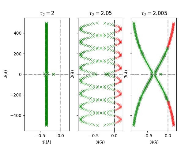
Example 2.6 from [Appeltans and Michiels, 2023] Section 2.3.2 demonstrates that the exponential stability of neutral systems might be fragile with respect to small delay perturbations.

Consider the following neutral delay differential equation (NDDE):

\[\dot{x}(t) = \frac{1}{4} x(t) - \frac{1}{3} x(t-\tau_1) + \frac{3}{4} \dot{x}(t-\tau_1) - \frac{1}{2} \dot{x}(t-\tau_2),\]

with \(\tau_1 = 1\) and \(\tau_2 = 2\). The associated delay differential equation is

\[x(t) - \frac{3}{4}x(t-\tau_1) + \frac{1}{2}x(t-\tau_2) = 0.\]

import matplotlib.pyplot as plt
import numpy as np
import tdcpy
import tdcpy.plot

A0 = np.array([[0.25]])
A1 = np.array([[-1./3]])

H1 = np.array([[-0.75]])
H2 = np.array([[0.5]])

r = [-0.9, 0.2, -500, 500]

fig, axes = plt.subplots(1, 3, sharex=True, sharey=True)

for delay, ax in zip([2, 2.05, 2.005], axes):
    ndde = tdcpy.NDDE(A=[A0, A1], hA=[0, 1], H=[H1, H2], hH=[1, delay])
    cr, info = tdcpy.roots(ndde, r=r, max_size_evp=1500)
    tdcpy.plot.eigen_plot(cr, ax=ax)
    ax.set_title(rf"$\tau_2={delay}$")

plt.show()