Example - strong stabilization

We consider the system described by the following delay-differential equation from [Michiels and Niculescu, 2007] and Example 3.2 of [Appeltans and Michiels, 2023]

\[\begin{split}\begin{aligned} \dot{x}(t) &= \begin{bmatrix} -0.08 & -0.03 & 0.2 \\ 0.2 & -0.04 & -0.005 \\ -0.06 & 0.2 & -0.07 \end{bmatrix} x(t) + \begin{bmatrix} -0.1 \\ -0.2 \\ 0.1 \end{bmatrix} u(t-5), \\ \\ y(t) &= \begin{bmatrix} 1 & 0 & 0 \\ 0 & 1 & 0 \\ 0 & 0 & 1 \\ \end{bmatrix} x(t) + \begin{bmatrix} 3. \\ 4. \\ 1. \end{bmatrix} u(t-2.5) + \begin{bmatrix} 0.4 \\ -0.4 \\ -0.4 \end{bmatrix} u(t-5). \end{aligned}\end{split}\]

with

\[u(t) = K y(t)\]

The goal is to compute the controller parameters K such that the closed-loop system is strongly stable.

We shall follow the following steps for designing our stabilizing controller:

1. Create the open-loop system as a DDAE object

2. Create the controller as a DDAE object and form the closed-loop

3. Optimize the controller parameters using controller_bfgs to minimize the spectral abscissa of the closed-loop system.

import numpy as np
import matplotlib.pyplot as plt

import tdcpy
from tdcpy import DDAE
import tdcpy.plot

Step 1: Create the open-loop DDAE

A0 = np.array([
    [   -0.08,  -0.03,  0.2     ],
    [   0.2,    -0.04,  -0.005  ],
    [   -0.06,  0.2,    -0.07    ],
])
Bu = np.array([
    [-0.1],
    [-0.2],
    [ 0.1],
])
C = np.array(np.eye(3)) # all states as outputs
D1 = np.array([
    [3],
    [4],
    [1],
])
D2 = np.array([[0.4], [-0.4], [-0.4]])
hD = np.array([2.5,5.])

plant = tdcpy.DDAE(
    A=[A0], hA=[0],
    B=[Bu], hB=[5.],
    C=[C], hC=[0],
    D=[D1, D2], hD=[2.5, 5],
)

print(plant)

<tdcpy.ddae.DDAE object at 0x7f58ddd69490>

Let us examine the open-loop system, is the system stable?

from tdcpy import spectral_abscissa
sa = spectral_abscissa(plant, r=-1)

print(f"Spectral abscissa of open-loop: {sa}")

Spectral abscissa of open-loop: 0.10805932731871844

Since the spectral abscissa is positive => the system is unstable. Let us try to stabilize it by static output feedback.

Step 2: Create the controller as a DDAE object and form the closed-loop

from tdcpy.common.closed_loop import controller_reprezentation
from tdcpy import ClosedLoop

E, K, hK = controller_reprezentation(order=0, n_inputs=3, n_outputs=1, hD=np.array([0.]))

cl = ClosedLoop(plant, order=0, y_indices=[0,1,2], u_indices=[0], K0=np.zeros_like(K), hK=hK)

/home/runner/work/tdcpy/tdcpy/src/tdcpy/common/closed_loop.py:67: SyntaxWarning: invalid escape sequence '\s'
  E x' = \sum_{k=0}^{hK} K_k x(t - hK_k)

Let us first check if the closed-loop is retarded or neutral

cl_ddae = DDAE(E=cl.E,A=cl.A,hA=cl.hA)          # extracting the closed-loop ddae
print(f"Is the closed-loop system retarded? {cl_ddae.is_essentially_retarded}")

Is the closed-loop system retarded? False

As the closed-loop is neutral, the controller will have to be designed for strong stability.

from tdcpy import strong_spectral_abscissa
ssa = strong_spectral_abscissa(cl_ddae, r=-1)

print(f"Strong spectral abscissa before optimization is: {ssa}")
region = [-0.5, 0.5, -0.5, 0.5]

cr_system, _ = tdcpy.roots(cl_ddae, r=region, discretization=100)
import matplotlib.pyplot as plt
import tdcpy.plot
fig, ax = plt.subplots()

tdcpy.plot.eigen_plot(cr_system, ax=ax)
ax.axvline(x=ssa, color="red", linestyle="--")
ax.text(ssa, 0, f"CD = {ssa:.4f}", color="red", fontsize=10,
        verticalalignment="bottom", horizontalalignment="right")
ax.legend()
ax.title = ax.set_title("Open-loop roots and strong spectral abscissa")
ax.set_xlim(region[0], region[1])
ax.set_ylim(region[2], region[3])
plt.show()

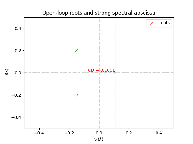
Strong spectral abscissa before optimization is: 0.10805932731871942

Step 3: Mimimizing the strong spectral abscissa of the closed-loop

To this end, the high-level function minimize_spectral_abscissa provides an interface for minimizing the strong spectral abscissa of the closed-loop system from function utilizes the minimize function from the scipy.optimize module. The default is the “L-BFGS-B” method.

from tdcpy.stabopt.controller_bfgs import design_bfgs, minimize_spectral_abscissa

options={'ftol': 1e-6, 'gtol': 1e-6}

sol = minimize_spectral_abscissa(plant, order=0, method="L-BFGS-B", options={"disp": True, **options}, callback=None, type = "barrier")

x = sol.x
K = x.reshape(K.shape)

# update the closed-loop with the optimized controller parameters
cl = tdcpy.ClosedLoop(plant, order=0, y_indices=[0,1,2], u_indices=[0], K0=K, hK=hK)
cl_ddae = DDAE(E=cl.E,A=cl.A,hA=cl.hA)          # extracting the closed-loop ddae

cd, cdInfo = tdcpy.spectral_abscissa_diff(cl_ddae, return_info=True)
ssa_cl = strong_spectral_abscissa(cl_ddae, r=-1)

print(f"Optimized cd = {cd}")
print(f"Strong spectral abscissa of closed-loop with L-BFGS-B = {ssa_cl}")

/home/runner/work/tdcpy/tdcpy/src/tdcpy/stabopt/controller_bfgs.py:511: SyntaxWarning: invalid escape sequence '\d'
  E \dot{x}(t) = (P_0 + B K_0 C) x(t) + \sum_{i=1}^{m} (P_i + B K_i C) x(t - \tau_i)
/home/runner/work/tdcpy/tdcpy/src/tdcpy/stabopt/gradients.py:209: SyntaxWarning: invalid escape sequence '\g'
  Computes the gradient of the function :math:`\gamma_0(p)` of the delay-difference
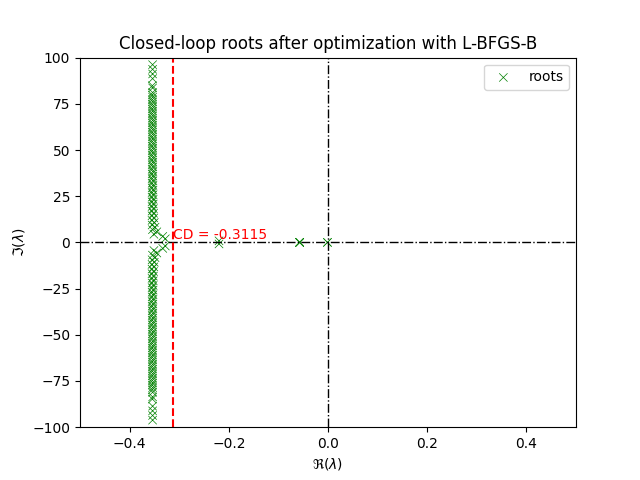
Optimized cd = -0.31150856756438117
Strong spectral abscissa of closed-loop with L-BFGS-B = -0.001118911790941013

Plotting the roots of the closed-loop system after optimization with L-BFGS-B

region = [-0.5, 0.5, -100, 100]
cr_cl, cr_info = tdcpy.roots(cl_ddae, r=-1, discretization=200)

fig, ax = plt.subplots()
tdcpy.plot.eigen_plot(cr_cl, ax=ax)
ax.axvline(x=cd, color="red", linestyle="--")
ax.text(cd, 0, f"CD = {cd:.4f}", color="red", fontsize=10,
        verticalalignment="bottom", horizontalalignment="left")
ax.legend()
title = ax.set_title("Closed-loop roots after optimization with L-BFGS-B")
ax.set_xlim(region[0], region[1])
ax.set_ylim(region[2], region[3])
plt.show()

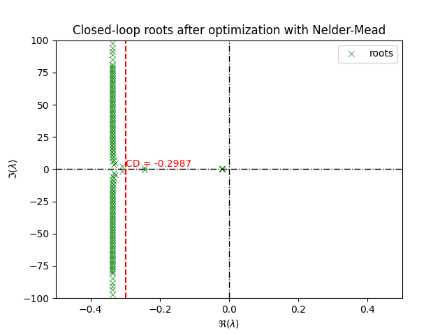
Although the spectral abscissa is minimized successfully, we can achieve better Due to the non-smoothness of the strong spectral abscissa, the L-BFGS-B solver can get stuck in a local minima. In order to achieve better results, we can try a different solver for example Nelder-Mead, which is a derivative-free solver and repeat the process

sol = minimize_spectral_abscissa(plant, order=0, method="Nelder-Mead", options={"disp": True, **options}, callback=None, type = "barrier")

x = sol.x
K = x.reshape(K.shape)

# update the closed-loop with the optimized controller parameters
cl = tdcpy.ClosedLoop(plant, order=0, y_indices=[0,1,2], u_indices=[0], K0=K, hK=hK)
cl_ddae = DDAE(E=cl.E,A=cl.A,hA=cl.hA)          # extracting the closed-loop ddae

# let us again compute the strong spectral abscissa of the closed-loop
cd, cdInfo = tdcpy.spectral_abscissa_diff(cl_ddae, return_info=True)
ssa_cl = strong_spectral_abscissa(cl_ddae, r=-1)

print(f"Optimized cd with Nelder-Mead = {cd}")
print(f"Strong spectral abscissa of closed-loop with Nelder-Mead = {ssa_cl}")

/home/runner/work/tdcpy/tdcpy/src/tdcpy/stabopt/controller_bfgs.py:419: RuntimeWarning: Method Nelder-Mead does not use gradient information (jac).
  sol = optimize.minimize(
/home/runner/work/tdcpy/tdcpy/src/tdcpy/stabopt/controller_bfgs.py:419: OptimizeWarning: Unknown solver options: ftol, gtol
  sol = optimize.minimize(
Optimization terminated successfully.
         Current function value: -0.000169
         Iterations: 88
         Function evaluations: 166
Optimization terminated successfully.
         Current function value: -0.017881
         Iterations: 190
         Function evaluations: 337
Optimization terminated successfully.
         Current function value: -0.018876
         Iterations: 59
         Function evaluations: 114
Optimization terminated successfully.
         Current function value: -0.019175
         Iterations: 59
         Function evaluations: 114
Optimization terminated successfully.
         Current function value: -0.019265
         Iterations: 59
         Function evaluations: 114
Optimization terminated successfully.
         Current function value: -0.019292
         Iterations: 59
         Function evaluations: 114
Optimization terminated successfully.
         Current function value: -0.019300
         Iterations: 59
         Function evaluations: 114
Optimization terminated successfully.
         Current function value: -0.019302
         Iterations: 59
         Function evaluations: 114
Optimization terminated successfully.
         Current function value: -0.019303
         Iterations: 59
         Function evaluations: 114
Optimization terminated successfully.
         Current function value: -0.019303
         Iterations: 59
         Function evaluations: 114
Optimized cd with Nelder-Mead = -0.298702954648969
Strong spectral abscissa of closed-loop with Nelder-Mead = -0.019303070354182772

Plotting the roots of the closed-loop system after optimization with Nelder-Mead

cr_cl, _ = tdcpy.roots(cl_ddae, r=-1, discretization=200)

fig, ax = plt.subplots()
tdcpy.plot.eigen_plot(cr_cl, ax=ax)
title = ax.set_title("Closed-loop roots after optimization with Nelder-Mead")
ax.set_xlim(region[0], region[1])
ax.set_ylim(region[2], region[3])
ax.axvline(x=cd, color="red", linestyle="--")
ax.text(cd, 0, f"CD = {cd:.4f}", color="red", fontsize=10,
        verticalalignment="bottom", horizontalalignment="left")
ax.legend()
plt.show()